3  Case study: gene expression data

Similarly, we load utility package tidyverse to help with data manipulation and visualization.

library(tidyverse)

In this demonstration, we use the curate Ovarian data (Ganzfried et al. 2013) to demonstrate (1) the common gene co-expression network drawn by \(\Sigma_\Phi\) and (2) the fit of the models via calculating MSE. This data contains the gene expression and clinical outcomes of 2970 patients collected from 23 studies. Different studies have different sequencing platforms, sample sizes, stage/subtype of the tumor, survival and censoring information.

3.1 Loading and previewing the data

We load the curatedOvarianData package to get the data. Description of each study can be found with data(package="curatedOvarianData").

library(curatedOvarianData)

#data(package="curatedOvarianData")
data(GSE13876_eset)
data(GSE26712_eset)
data(GSE9891_eset)
data(PMID17290060_eset)

The four datasets are of similar sizes. All of them have the majority of patients in the late stage of the cancer, and histological subtypes observed in the tissue samples are mostly serous carcinoma. The datasets differs in respect sequencing platforms, which are Operonv3two-color, AffymetrixHG-U133A, AffymetrixHG-U133Plus2 and AffymetrixHG-U133A.

3.2 Data pre-processing

First we find intersection of genes that are exist in all four studies. We use featureNames to extract the gene names and exprs to extract the data matrices. More operations of the ExpressionSets can be found in (Falcon, Morgan, and Gentleman 2007).

inter_genes <- Reduce(intersect, list(featureNames(GSE13876_eset),
                                      featureNames(GSE26712_eset), 
                                      featureNames(GSE9891_eset),
                                      featureNames(PMID17290060_eset)))

GSE13876_eset <- GSE13876_eset[inter_genes,]
GSE26712_eset <- GSE26712_eset[inter_genes,]
GSE9891_eset <- GSE9891_eset[inter_genes,]
PMID17290060_eset <- PMID17290060_eset[inter_genes,]

study1 <- t(exprs(GSE13876_eset))
study2 <- t(exprs(GSE26712_eset))
study3 <- t(exprs(GSE9891_eset))
study4 <- t(exprs(PMID17290060_eset))

We then filter the genes so that only high variance genes are kept for later analysis.

# calculate Coefficient of Variation of each gene
cv1 <- apply(study1, 2, sd) / apply(study1, 2, mean)
cv2 <- apply(study2, 2, sd) / apply(study2, 2, mean)
cv3 <- apply(study3, 2, sd) / apply(study3, 2, mean)
cv4 <- apply(study4, 2, sd) / apply(study4, 2, mean)
cv_matrix <- rbind(cv1, cv2, cv3, cv4)

# Find genes with CV >= threshold in at least one study
threshold <- 0.16
genes_to_keep <- apply(cv_matrix, 2, function(cv) any(cv >= threshold))
sum(genes_to_keep)

[1] 1060

# Filtered
study1 <- GSE13876_eset[genes_to_keep,]
study2 <- GSE26712_eset[genes_to_keep,]
study3 <- GSE9891_eset[genes_to_keep,]
study4 <- PMID17290060_eset[genes_to_keep,]

Next, we log-transform the data (for a better normality) and store them in 4 \(N_s\times P\) matrices.

df1 <- study1 %>% exprs() %>% t() %>% 
  log() %>% as.data.frame()
df2 <- study2 %>% exprs() %>% t() %>% 
  log() %>% as.data.frame()
df3 <- study3 %>% exprs() %>% t() %>% 
  log()  %>% as.data.frame()
df4 <- study4 %>% exprs() %>% t() %>% 
  log()  %>% as.data.frame()
list_gene <- list(df1, df2, df3, df4)
saveRDS(list(df1, df2, df3, df4), "./Data/CuratedOvarian_processed.rds")

Now we can see the dimensions of each study:

sapply(list_gene, dim)

     [,1] [,2] [,3] [,4]
[1,]  157  195  285  117
[2,] 1060 1060 1060 1060

The ultimate data for analysis has \(N_s=(157, 195, 285, 117)\) for \(s=1,2, 3, 4\), and \(P=1060\).

We scale the data so that we focus on the correlations between the genes. When the data are scaled, the variance of the genes are 1 and the off-diagonal values scales up, so does the estimated covariances matrices, which facilitates a more interpretable network analysis.

Y_list <- readRDS("./Data/CuratedOvarian_processed.rds")
Y_list_scaled <- lapply(
 Y_list, function(x) scale(x, center = TRUE, scale = TRUE)
)
Y_mat_scaled <- Y_list_scaled %>% do.call(rbind, .) %>% as.matrix()

3.3 Fitting the models

For models fitted with MSFA::sp_fa, the function provides scaling and centering arguments. Therefore, we do not need to use the scaled data before fitting (here I use Mavis’s version of MSFA).

Stack FA and Ind FA:

Y_mat =  Y_list %>% do.call(rbind, .) %>% as.matrix()
fit_stackFA <- MSFA::sp_fa(Y_mat, k = 6, scaling = FALSE, centering = TRUE, 
                                control = list(nrun = 10000, burn = 8000))

fit_indFA <-
      lapply(1:6, function(s){
        j_s = c(8, 8, 8, 8, 8, 8)
        MSFA::sp_fa(Y_list[[s]], k = j_s[s], scaling = FALSE, centering = TRUE,
                    control = list(nrun = 10000, burn = 8000))
      })

MOM-SS:

# Construct the membership matrix
N_s <- sapply(Y_list, nrow)
M_list <- list()
   for(s in 1:4){
     M_list[[s]] <- matrix(1, nrow = N_s[s], ncol = 1)
   }
M <- as.matrix(bdiag(M_list))

fit_MOMSS <- BFR.BE::BFR.BE.EM.CV(x = Y_mat, v = NULL, b = M, q = 20, scaling = TRUE)

PFA (we don’t recommend running it. It takes 4 days and more.)

N_s <- sapply(Y_list, nrow)
fit_PFA <- PFA(Y=t(Y_mat_scaled), 
                        latentdim = 20,
                       grpind = rep(1:4, 
                                     times = N_s),
              Thin = 5,
              Cutoff = 0.001,
              Total_itr = 10000, burn = 8000)

SUFA (takes about 10 hours):

fit_SUFA <- SUFA::fit_SUFA(Y_list_scaled, qmax=20,nrun = 10000)

BMSFA:

fit_BMSFA <- MSFA::sp_msfa(Y_list, k = 20, j_s = c(4, 4, 4, 4),
                              outputlevel = 1, scaling = TRUE, centering = TRUE, 
                               control = list(nrun = 10000, burn = 8000))

Tetris (we don’t recommend running it. It could take more than 10 days.):

set_alpha <- ceiling(1.25*4)
fit_Tetris <- tetris(Y_list_scaled, alpha=set_alpha, beta=1, nprint = 200, nrun=10000, burn=8000)
print("Start to choose big_T. It might take a long time.")
big_T <- choose.A(fit_Tetris, alpha_IBP=set_alpha, S=4)
run_fixed <- tetris(Y_list_scaled, alpha=set_alpha, beta=1, 
                     fixed=TRUE, A_fixed=big_T, nprint = 200, nrun=10000, burn=8000)

3.4 Post-processing

We use the post_xxx() functions defined in the chapter of nutrition applications to post-process for point estimates of the factor loadings, common factors, and covariance matrices.

For Stack FA, Ind FA and BMSFA, we need to determine the number of common factors \(K\) and the number of latent dimensions \(J_s\) for each study after the post-processing, and we need to re-run those models.

Here we start with Stack FA, Ind FA and BMSFA:

# Stack FA
res_stackFA = post_stackFA(fit_stackFA, S=4)
# Ind FA
res_IndFA = post_IndFA(fit_indFA)
# BMSFA
res_BMSFA = post_BMSFA(fit_BMSFA)

# Eigenvalue decomposition
fun_eigen <- function(Sig_mean) {
  val_eigen <- eigen(Sig_mean)$values
  prop_var <- val_eigen/sum(val_eigen)
  choose_K <- length(which(prop_var > 0.05))
  return(choose_K)
}

SigmaPhi_StackFA <- res_stackFA$SigmaPhi
K_StackFA <- fun_eigen(SigmaPhi_StackFA)

SigmaLambda_IndFA <- res_IndFA$SigmaLambda
Js_IndFA <- lapply(SigmaLambda_IndFA, fun_eigen)

SigmaPhi_BMSFA <- res_BMSFA$SigmaPhi
K_BMSFA <- fun_eigen(SigmaPhi_BMSFA)
SigmaLambda_BMSFA <- res_BMSFA$SigmaLambda
Js_BMSFA <- lapply(SigmaLambda_BMSFA, fun_eigen)

# We print the results:
print(paste0("Stack FA: K = ", K_StackFA))

[1] "Stack FA: K = 2"

print(paste0("Ind FA: J_s = ", Js_IndFA))

[1] "Ind FA: J_s = 4" "Ind FA: J_s = 7" "Ind FA: J_s = 6" "Ind FA: J_s = 6"

print(paste0("BMSFA: K = ", K_BMSFA))

[1] "BMSFA: K = 6"

print(paste0("BMSFA: J_s = ", Js_BMSFA))

[1] "BMSFA: J_s = 4" "BMSFA: J_s = 4" "BMSFA: J_s = 4" "BMSFA: J_s = 4"

We then fit the models again with the determined number of factors and latent dimensions.

# Stack FA
fit_stackFA2 <- MSFA::sp_fa(Y_mat, k = K_StackFA, scaling = FALSE, centering = TRUE, 
                                control = list(nrun = 10000, burn = 8000))
# Ind FA
fit_indFA2 <- lapply(1:4, function(s){
  j_s = Js_IndFA[[s]]
  MSFA::sp_fa(Y_list[[s]], k = j_s, scaling = FALSE, centering = TRUE,
              control = list(nrun = 10000, burn = 8000))
})
# BMSFA
fit_BMSFA2 <- MSFA::sp_msfa(Y_list, k = K_BMSFA, j_s = Js_BMSFA,
                            outputlevel = 1, scaling = TRUE, centering = TRUE, 
                            control = list(nrun = 10000, burn = 8000))

# Again we post-process the MCMC chains.
res_stackFA2 <- post_stackFA(fit_stackFA2, S=4)
res_IndFA2 <- post_IndFA(fit_indFA2)
res_BMSFA2 <- post_BMSFA(fit_BMSFA2)

For the rest of the methods, we apply the same post-processing functions as in the nutrition applications chapter.

# PFA
res_PFA <- post_PFA(fit_PFA)
# MOM-SS
res_MOMSS <- post_MOMSS(fit_MOMSS)
# SUFA
res_SUFA <- post_SUFA(fit_SUFA)
# Tetris
#res_Tetris <- post_Tetris(fit_Tetris)

3.5 Visualization

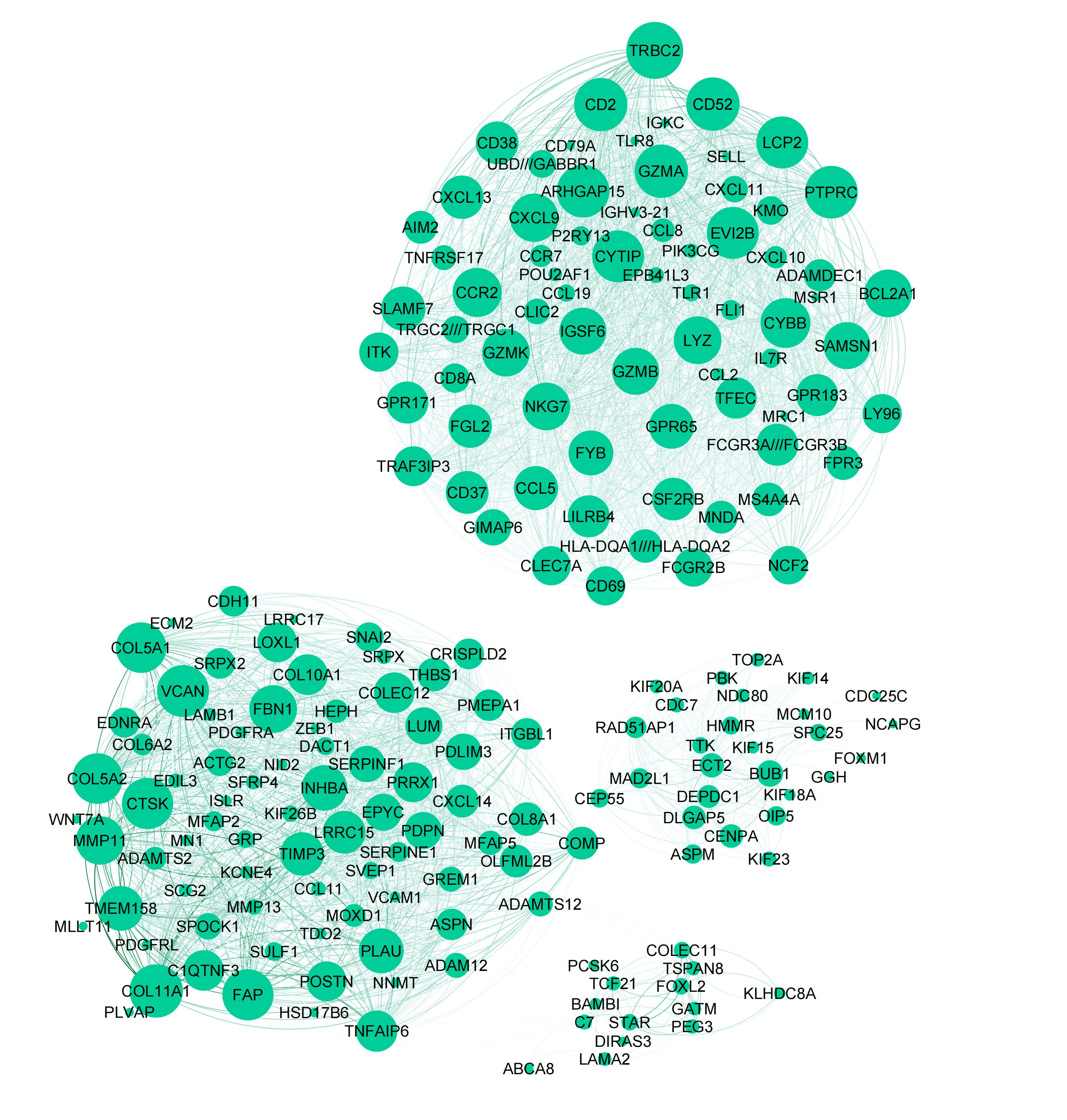
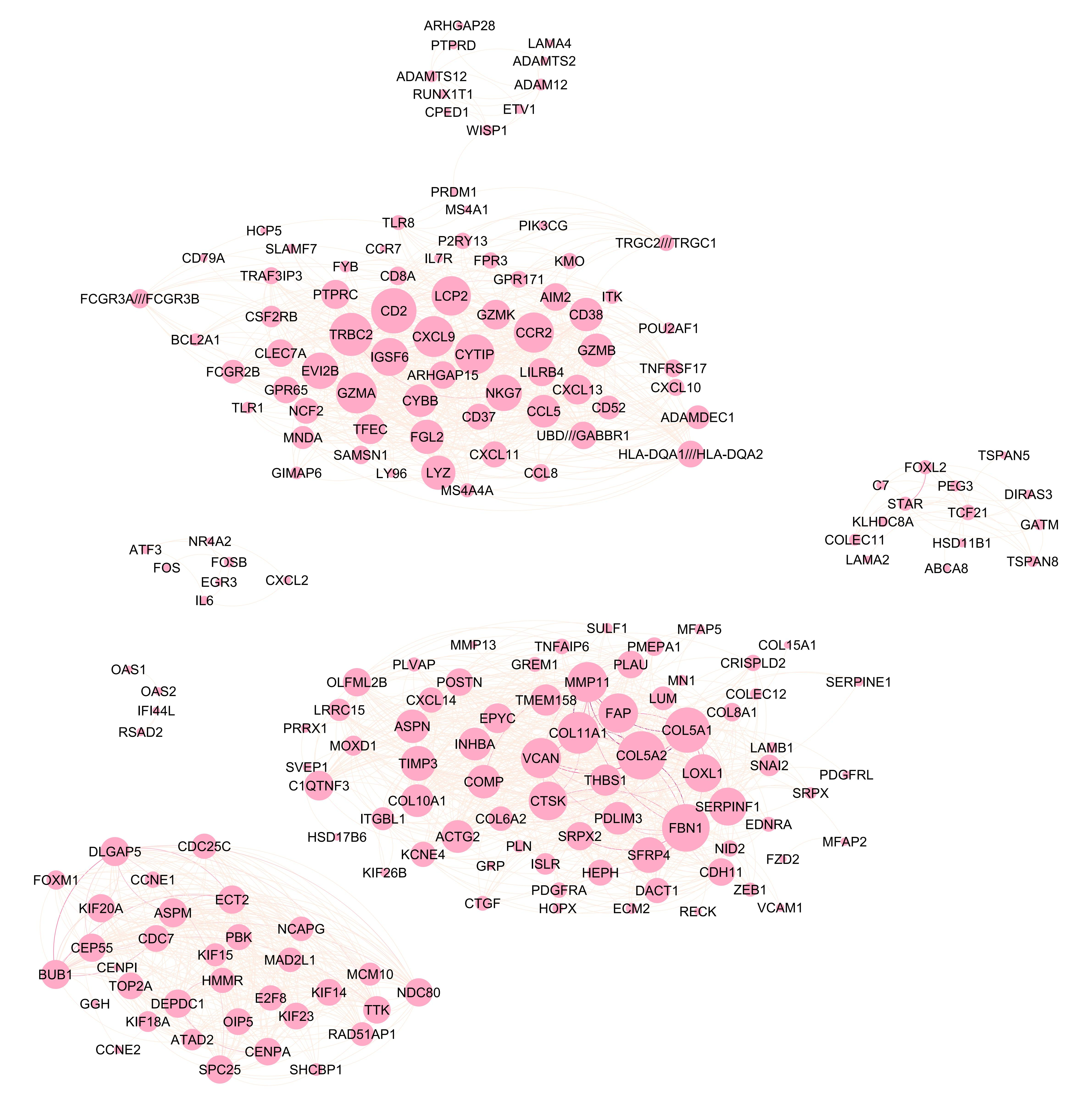
We can visualize the common gene co-expression network using the estimated common covariance matrices. We use Gephi to visualize the networks. The SigmaPhi matrix is the common covariance matrix, and SigmaLambda is the study-specific covariance matrix.

Before that, we need to filter the genes so that only genes with high correlations are kept (leaving around 200 genes in the plot). We set the threshold for each model as follows:

• Stack FA: 0.85
• MOM-SS: 0.95
• BMSFA: 0.5
• SUFA: 0.28
• PFA: 0.55

# Filtering genes for visualization in Gephi
genenames <- colnames(list_gene[[1]])

# StackFA
SigmaPhi_StackFA_curated <- res_stackFA2$SigmaPhi
colnames(SigmaPhi_StackFA_curated) <- rownames(SigmaPhi_StackFA_curated) <- genenames
diag(SigmaPhi_StackFA_curated) <- NA
above_thresh <- SigmaPhi_StackFA_curated > 0.85
keep_genes <- apply(above_thresh, 1, function(x) any(x, na.rm = TRUE))
sum(keep_genes)

[1] 214

SigmaPhi_StackFA_curated[abs(SigmaPhi_StackFA_curated) < 0.85] <- 0
SigmaPhi_StackFA_curated_filtered <- SigmaPhi_StackFA_curated[keep_genes, keep_genes]
#write.csv(SigmaPhi_StackFA_curated_filtered, "SigmaPhi_StackFA_curated_filtered.csv")

# MOM-SS
SigmaPhiMOMSS <- res_MOMSS$SigmaPhi
colnames(SigmaPhiMOMSS) <- rownames(SigmaPhiMOMSS) <- genenames
diag(SigmaPhiMOMSS) <- NA
above_thresh <- abs(SigmaPhiMOMSS) > 0.95
keep_genes <- apply(above_thresh, 1, function(x) any(x, na.rm = TRUE))
sum(keep_genes)

[1] 223

SigmaPhiMOMSS[abs(SigmaPhiMOMSS) < 0.95] <- 0
SigmaPhiMOMSS_filtered <- SigmaPhiMOMSS[keep_genes, keep_genes]
#write.csv(SigmaPhiMOMSS_filtered, "SigmaPhiMOMSS_filtered.csv")

# BMSFA
SigmaPhiBMSFA <- res_BMSFA2$SigmaPhi
colnames(SigmaPhiBMSFA) <- rownames(SigmaPhiBMSFA) <- genenames
diag(SigmaPhiBMSFA) <- NA
above_thresh <- abs(SigmaPhiBMSFA)  > 0.5
keep_genes <- apply(above_thresh, 1, function(x) any(x, na.rm = TRUE))
sum(keep_genes)

[1] 192

SigmaPhiBMSFA[abs(SigmaPhiBMSFA) < 0.5] <- 0
SigmaPhiBMSFA_filtered <- SigmaPhiBMSFA[keep_genes, keep_genes]
#write.csv(SigmaPhiBMSFA_filtered, "SigmaPhiBMSFA_filtered.csv")

# SUFA
SigmaPhiSUFA <- res_SUFA$SigmaPhi
colnames(SigmaPhiSUFA) <- rownames(SigmaPhiSUFA) <- genenames
diag(SigmaPhiSUFA) <- NA
above_thresh <- abs(SigmaPhiSUFA) > 0.28
keep_genes <- apply(above_thresh, 1, function(x) any(x, na.rm = TRUE))
sum(keep_genes)

[1] 191

SigmaPhiSUFA[abs(SigmaPhiSUFA) < 0.28] <- 0
SigmaPhiSUFA_filtered <- SigmaPhiSUFA[keep_genes, keep_genes]
#write.csv(SigmaPhiSUFA_filtered, "SigmaPhiSUFA_filtered.csv")

# PFA
SigmaPhiPFA <- res_PFA$SigmaPhi
colnames(SigmaPhiPFA) <- rownames(SigmaPhiPFA) <- genenames
diag(SigmaPhiPFA) <- NA
above_thresh <- abs(SigmaPhiPFA) > 0.55
keep_genes <- apply(above_thresh, 1, function(x) any(x, na.rm = TRUE))
sum(keep_genes)

[1] 203

SigmaPhiPFA[abs(SigmaPhiPFA) < 0.55] <- 0
SigmaPhiPFA_filtered <- SigmaPhiPFA[keep_genes, keep_genes]
#write.csv(SigmaPhiPFA_filtered, "SigmaPhiPFA_filtered.csv")

Attached are the final figures make with Gephi. The nodes are the genes and the edges are the correlations between the genes. The thickness of the edges indicates the strength of the correlation. The color of the nodes indicates the study they belong to. The size of the nodes indicates the number of connections they have.

Stack FA:

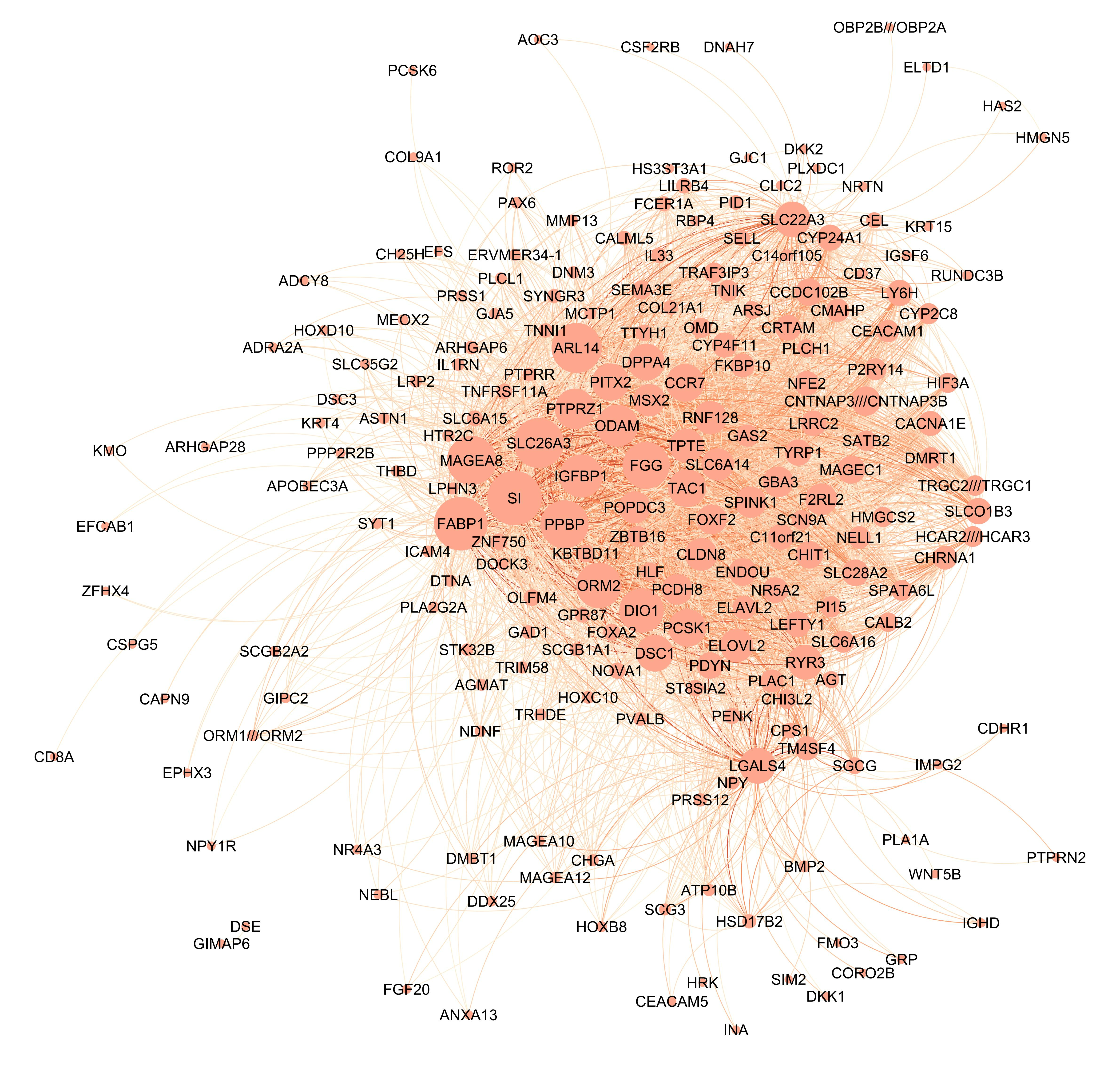
PFA:

MOM-SS:

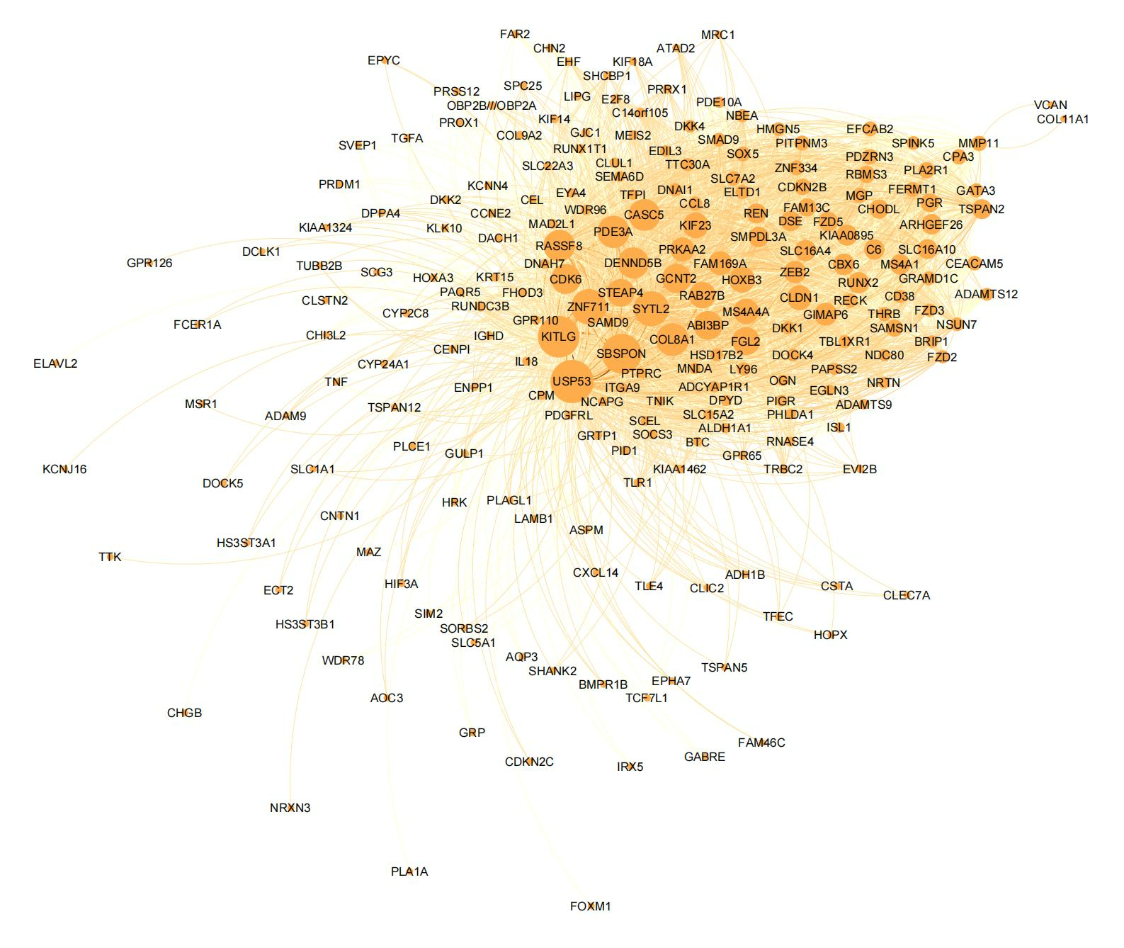
SUFA:

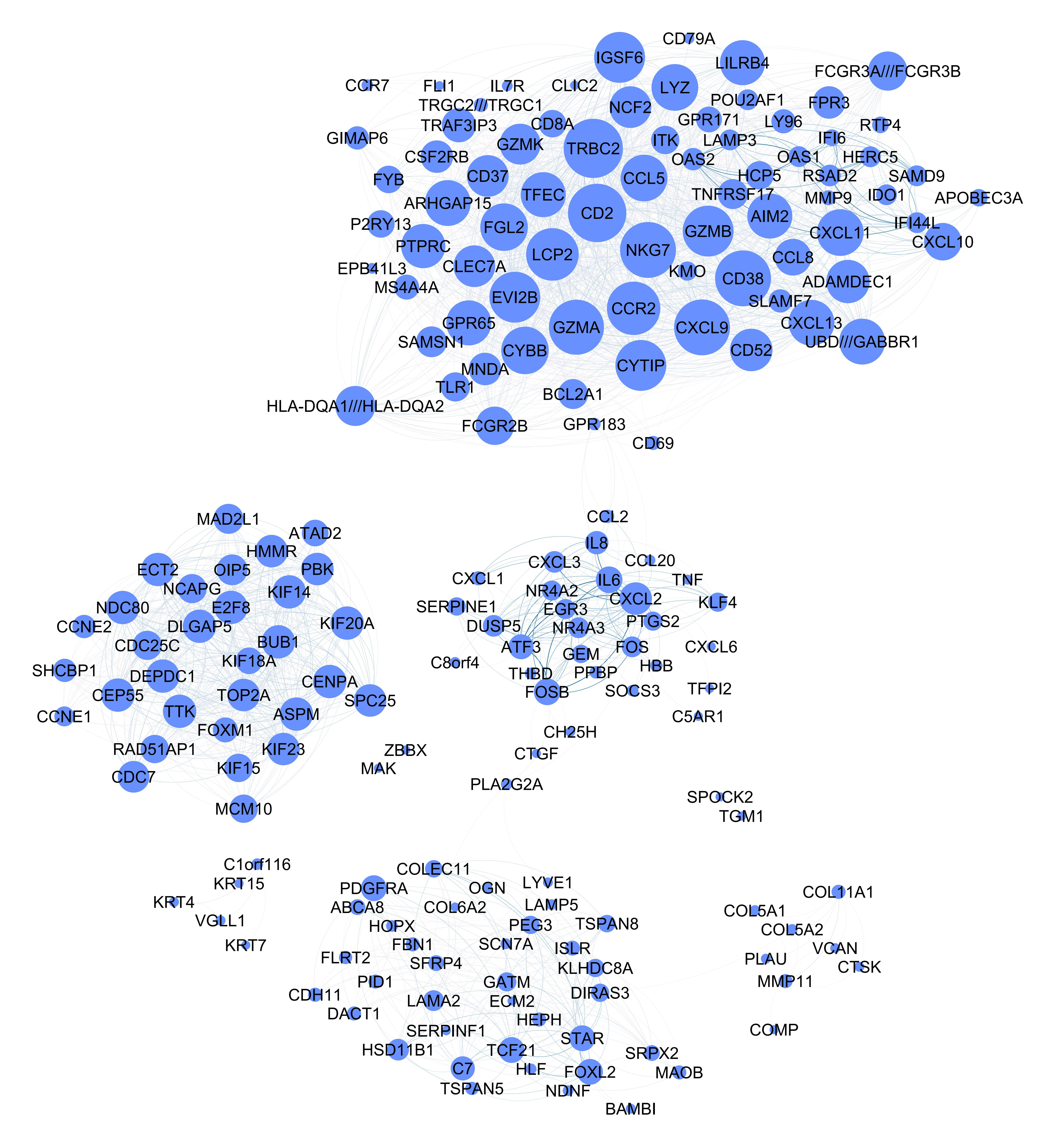
BMSFA:

Falcon, Seth, Martin Morgan, and Robert Gentleman. 2007. “An Introduction to Bioconductor’s Expressionset Class.”

Ganzfried, Benjamin Frederick, Markus Riester, Benjamin Haibe-Kains, Thomas Risch, Svitlana Tyekucheva, Ina Jazic, Xin Victoria Wang, et al. 2013. “curatedOvarianData: Clinically Annotated Data for the Ovarian Cancer Transcriptome.” Database 2013.